Getting started

Getting started¶

Installation¶

To install ScattPy one needs:

Python 2.5 - 2.7
F2PY with a configured FORTRAN77 compiler
Python packages:
- NumPy
- SciPy
- NumdiffTools

Ubuntu¶

$ sudo apt-get install python-numpy python-scipy python-dev python-setuptools ipython
$ sudo easy_install numdifftools
$ sudo easy_install scikits.scattpy

Windows¶

Instructions for installing ScattPy under Windows operating system will be added later

Sample Session¶

The most simple way of trying ScattPy is to run an interactive python session with IPython.

$ ipython

Import required packages.

In [2]: from numpy import * ;
In [3]: from scikits.scattpy import * ;

Define a prolate spheroidal particle with the size parameter $x_{\rm V}=2$ , aspect ratio $a/b=4$ and complex refractive index $m$ .

In [4]: P = ProlateSpheroid(ab=4., xv=2., m=1.33+0.2j)

Define a laboratory object that desribes the incident wave and the scatterer. We will consider a plane wave propagating at the angle $\alpha=\pi/4$ to the particle symmetry axis.

In [5]: LAB = Lab(P, alpha=pi/4)

Now we can use any of the ScattPy’s numerical methods to obtain scattering properties of the defined model. In this example we apply the extended boundary conditions method (EBCM) that is best suited for homogeneous spheroids.

In [6]: RES = ebcm(LAB)

************************************************************
m1=1, alpha=45.0
homogeneous prolate spheroid with ab=4.0, xv=2.0, m=(1.33+0.2j)

************************************************************
N 		 err TM		 err TE
4		 4.3e-01	 3.1e-01
6		 3.6e-01	 3.5e-01
8		 4.3e-02	 1.5e-02
10		 5.8e-03	 9.6e-03
12		 6.6e-04	 1.5e-04
14		 8.3e-06	 4.3e-05
16		 2.6e-06	 2.5e-06
18		 1.4e-05	 1.5e-05
20		 1.1e-04	 1.9e-04
22		 7.4e-04	 1.2e-03
Terminating: no more convergence expected
TM mode: Qext=1.6146281660410078e+00 , Qsca=5.6870956836659525e-01, delta=2.6e-06 , n=16
TE mode: Qext=1.3324784863705399e+00 , Qsca=4.8906404506136369e-01, delta=2.5e-06 , n=16

The returned RES object contains the expansion coefficients of the scattered field for the TM and TE modes. These coefficients can be used to obtain optical characteristics such as scattering cross-sections and efficiency factors

In [7]: Csca_tm,Qsca_tm = LAB.get_Csca(RES.c_sca_tm) ;
In [8]: print Csca_tm,Qsca_tm
7.14661520803 0.568709568367

One can also calculate amplitude ans scattering matrix elements for defined ranges of scattering angles, e.g. $\Theta\in[0,\pi],\;\varphi=0$ :

In [9]: Theta = linspace(0,pi,1000) ;
In [10]: A = LAB.get_amplitude_matrix(RES.c_sca_tm,RES.c_sca_te,Theta,0) ;
In [11]: S11g,S21_S11 = LAB.get_int_plr(A) ;

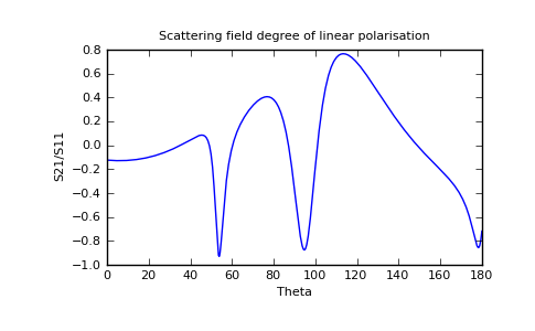
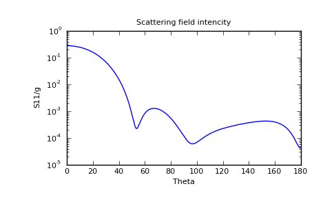
Using ScattPy together with Python data visualisation packages one can obtain plots of the scattering matrix elements.

In [12]: from matplotlib import pylab

In [13]: pylab.semilogy(Theta*180/pi, S11g);
In [14]: pylab.ylabel("S11/g");
In [15]: pylab.xlabel("Theta");
In [16]: pylab.title("Scattering field intencity");
In [17]: pylab.show()

In [23]: pylab.close()

In [24]: pylab.plot(Theta*180/pi, S21_S11);
In [25]: pylab.ylabel("S21/S11");
In [26]: pylab.xlabel("Theta");
In [27]: pylab.title("Scattering field degree of linear polarisation");
In [28]: pylab.show()

ScattPy

Navigation